Orbit-by-Orbit Plots
Plotting a series of orbit-by-orbit plots is a great way to become familiar
with a satellite data set. If the data set doesn’t come with orbit information
this can be a challenge. Orbits also go past day breaks. If data comes in daily
files this requires loading multiple files at once, joining the data together,
etc. pysat goes through that trouble for you. This code is available in
the pysat repository at demo/cnofs_vefi_dc_b_orbit_plots.py.
import datetime as dt
from matplotlib import ticker
import matplotlib.pyplot as plt
import os
import pysat
import pysatNASA

# Set the directory where the plots will be saved. Setting nothing will put
# the plots in the current directory
results_dir = ''

# Select C/NOFS VEFI DC magnetometer data, use longitude to determine where
# there are changes in the orbit (local time info not in file)
orbit_info = {'index': 'longitude', 'kind': 'longitude'}
vefi = pysat.Instrument(inst_module=pysatNASA.instruments.cnofs_vefi,
                        tag='dc_b', clean_level='none',
                        orbit_info=orbit_info)

# Set limits on dates analysis will cover, inclusive
start = dt.datetime(2010, 5, 9)
stop = dt.datetime(2010, 5, 12)

# If the desired data is not on your system, run the download commmand
if vefi.files[start:stop].shape[0] < (stop - start).days:
    vefi.download(start, stop)

# Specify the analysis time limits using `bounds`, otherwise all VEFI DC
# data will be processed
vefi.bounds = (start, stop)

# For each loop pysat puts a copy of the next available orbit into
# `vefi.data`. Changing .data at this level does not alter other orbits.
# Reloading the same orbit will erase any changes made
for orbit_count, vefi in enumerate(vefi.orbits):
    # Satellite data can have time gaps, which leads to plots with erroneous
    # lines connecting measurements on both sides of the gap if you plot the
    # data using lines instead of markers. The command below fills in any
    # data gaps using a 1-second cadence with NaNs, which Python will treat
    # as a gap when plotting with lines or markers. See the matplotlib
    # documentation for more information about plotting behavior and the
    # pandas documentation for more information about the `resample` mtehod.
    # The 1-s cadence was chosen because it is the nominal cadence for this
    # instrument.
    vefi.data = vefi.data.resample('1s', label='left').ffill(limit=1)

    # Create a figure with seven subplots
    fig, ax = plt.subplots(7, sharex=True, figsize=(8.5, 11))

    # Plot the data for each subplot
    p_params = ['B_flag', 'B_north', 'B_up', 'B_west', 'dB_mer', 'dB_par',
                'dB_zon']
    for i, pax in enumerate(ax):
        if i == 0:
            bwidth = (vefi['longitude'][-1] - vefi['longitude'][0]) / (
                vefi.data.index[-1] - vefi.data.index[0]).total_seconds()
            pax.bar(vefi['longitude'], vefi[p_params[i]] + 0.5,
                    width=bwidth, bottom=-0.5)
            pax.set_title(' - '.join((vefi.data.index[0].ctime(),
                                      vefi.data.index[-1].ctime())))
            pax.set_ylabel('Interp. Flag')
            pax.set_ylim(-0.5, 1.5)
        else:
            pax.plot(vefi['longitude'], vefi[p_params[i]], '-', lw=0.5)
            pax.set_title(vefi.meta[p_params[i]].name)
            pax.set_ylabel(vefi.meta[p_params[i]].units)

        if i == 6:
            pax.set_xlabel(vefi.meta['longitude'].name)
            pax.xaxis.set_major_formatter(ticker.FormatStrFormatter('%d'))
        else:
            pax.xaxis.set_major_formatter(ticker.FormatStrFormatter(''))
        pax.xaxis.set_major_locator(ticker.MultipleLocator(60))

    # Format and save the output for this orbit
    fig.tight_layout()
    plot_name = 'orbit_{num:05}.png'.format(num=orbit_count)
    fig.savefig(os.path.join(results_dir, plot_name))
    plt.close()
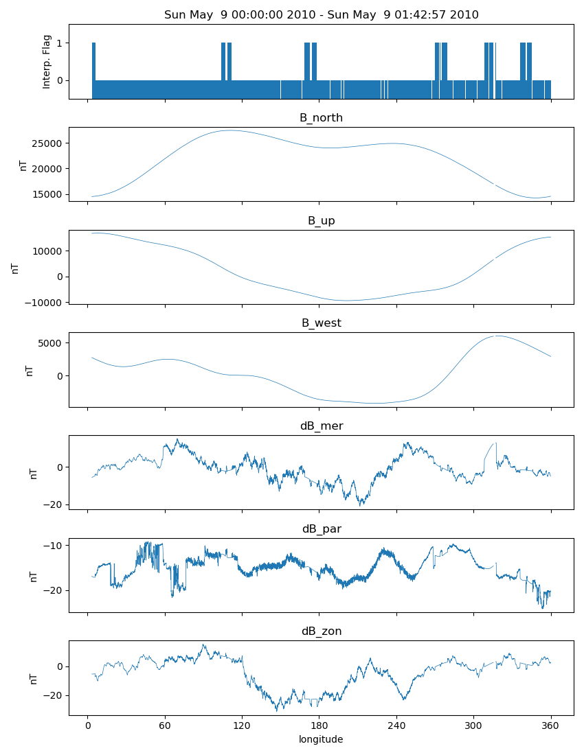
This will create 56 files with data from each orbit. Sample output from the first orbit is shown below.